Quickstart
This page gives an introduction in how to get started with LEMON, showing the steps that would normally be necessary to reduce a data set. In particular, this example assumes that we have a series of FITS images from a transit of exoplanet WASP-10b.
Important
Your data is assumed to be calibrated. Bias and dark subtraction, flat-fielding correction and any other necessary steps should have been performed before any data is fed to the pipeline.
Let’s take a look at each of the steps of the data reduction.
Do astrometry
Your FITS images need to be astrometrically solved before we can do
photometry. The astrometry command takes multiple FITS files as
input and writes a copy of them, containing the WCS header, to the
output directory specified in the last argument.
$ lemon astrometry data/*.fits WASP10/
>> The output directory 'WASP10' did not exist, so it had to be created.
>> Using a local build of Astrometry.net.
>> Doing astrometry on the 193 paths given as input.
>> 100%[======================================================================>]
>> You're done ^_^
As all LEMON commands, astrometry spawns multiple processes in
order to fully leverage all the processors your machine has. This
usually results in significant speed-ups on multi-core systems. If
that is not your case, this can always be modified via the --cores
option.
The astrometry command is built on top of Astrometry.net.
Mosaic the data
Now that the FITS images are astrometrically calibrated, let’s reproject them onto a common
coordinate system and combine them into a mosaic. The mosaic
command takes multiple FITS as input and combines them. The last
argument that it receives is the name of the file to which the
resulting image is written.
$ lemon mosaic WASP10/*.fits WASP10-mosaic.fits
>> Making sure the 193 input paths are FITS images...
>> 100%[======================================================================>]
INFO: Listing raw frames [montage_wrapper.wrappers]
INFO: Computing optimal header [montage_wrapper.wrappers]
INFO: Projecting raw frames [montage_wrapper.wrappers]
INFO: Mosaicking frames [montage_wrapper.wrappers]
INFO: Deleting work directory [montage_wrapper.wrappers]
>> Reproject mosaic to point North... done.
>> You're done ^_^
It is worth mentioning --background-match, an option which removes
any discrepancies in the brightness or background of the FITS images
before mosaicking them. Although a rather powerful feature, it is
disabled by default as it makes the assembling of the images take
remarkably longer and requires much more storage for the temporary
files it generates.
The mosaic command is built on top of Montage.
Do photometry
The mosaic that we have created is the image in which our astronomical objects are detected. As it maximizes the signal-to-noise ratio, this allows for a much more accurate determination of the centroid of each star, galaxy or any other celestial object.
The photometry command does aperture photometry on all the FITS
images that it receives as argument, using the first one to detect the
astronomical objects to measure. The last argument is the filename of
the LEMON database where the photometric measurements are stored.
$ lemon photometry WASP10-mosaic.fits WASP10/*.fits WASP10-phot.LEMONdB
>> Examining the headers of the 193 FITS files given as input...
>> 100%[======================================================================>]
>> 2 different photometric filters were detected:
>>  B: 16 files (8.29 %)
>>  V: 177 files (91.71 %)
>> Making sure there are no images with the same date and filter... done.
>> Sources image: WASP10-mosaic.fits
>> Running SExtractor on the sources image... done.
>> Calculating coordinates of field center... done.
>> α = 349.0447049  (23 16 10.73)
>> δ =  31.4843645 (+31 29 03.71)
>> Detected 155 sources on which to do photometry.
>>
>> Need to determine the instrumental magnitude of each source.
>> Doing photometry on the sources image, using the parameters:
>> FWHM (sources image) = 8.535 pixels, therefore:
>> Aperture radius = 8.535 x 3.00 = 25.605 pixels
>> Sky annulus, inner radius = 8.535 x 4.50 = 38.407 pixels
>> Sky annulus, width = 8.535 x 1.00 = 8.535 pixels
>>
>> Running IRAF's qphot... done.
>> Detecting INDEF objects... done.
>> 9 objects are INDEF in the sources image.
>> There are 146 objects left on which to do photometry.
>> Making sure INDEF objects were removed... done.
>>
>> Initializing output LEMONdB... done.
>>
>> Let's do photometry on the 16 images taken in the B filter.
>> Calculating the median FWHM for this filter... done.
>> FWHM (B) = 9.815 pixels, therefore:
>> Aperture radius = 9.815 x 3.00 = 29.445 pixels
>> Sky annulus, inner radius = 9.815 x 4.50 = 44.168 pixels
>> Sky annulus, width = 9.815 x 1.00 = 9.815 pixels
>> 100%[======================================================================>]
>>
>> Let's do photometry on the 177 images taken in the V filter.
>> Calculating the median FWHM for this filter... done.
>> FWHM (V) = 9.864 pixels, therefore:
>> Aperture radius = 9.864 x 3.00 = 29.592 pixels
>> Sky annulus, inner radius = 9.864 x 4.50 = 44.388 pixels
>> Sky annulus, width = 9.864 x 1.00 = 9.864 pixels
>> 100%[======================================================================>]
>> Storing photometric measurements in the database...
>> 100%[======================================================================>]
>> Gathering statistics about tables and indexes... done.
>> You're done ^_^
For each photometric filter, the aperture radius and sky annulus are
determined by the median FWHM of
all the images taken in that filter. This provides a robust value
that should work well in most scenarios, but if the atmospheric
conditions in your data vary considerably you may want to use
--individual. This makes the aperture and annulus be determined by
the FWHM of each image.
If instead of doing photometry on all the astronomical objects in the
field you only need to measure some of them, use --coordinates.
This option takes the path to a text file listing, one per line, the
celestial coordinates of the objects to measure.
The photometry command is built on top of IRAF and SExtractor.
Generate the light curves
The diffphot command takes a LEMON database with the
photometric measurements and computes the
differential light curve of each astronomical object in each of the
filters in which it was observed. The second argument is the name of
the output LEMON database to which to store the light curves, as well
as a copy of all the information present in the input database.
$ lemon diffphot WASP10-phot.LEMONdB WASP10-diff.LEMONdB
>> Making a copy of the input database... done.
>> There are 146 stars in the database
>>
>> Light curves for the B filter will now be generated.
>> Loading photometric information... done.
>> 100%[======================================================================>]
>> Storing the light curves in the database...
>> 100%[======================================================================>]
>>
>> Light curves for the V filter will now be generated.
>> Loading photometric information... done.
>> 100%[======================================================================>]
>> Storing the light curves in the database...
>> 100%[======================================================================>]
>> Updating statistics about tables and indexes... done.
>> You're done ^_^
The algorithm, our implementation of that described in
2005AN….326..134B, computes an optimal artificial comparison star
for each of our astronomical objects, identifying those that are the
most constant and assigning them weights inversely proportional to
their statistical dispersion. This is an iterative process that, at
each step, discards the --worst-fraction objects until only the
best ones remain. These are then combined into the artificial
comparison star.
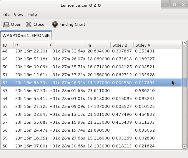
View the results
To view and analyze the light-curves,
open the LEMONdB with juicer:
$ lemon juicer WASP10-diff.LEMONdB
This opens a window listing all the astronomical objects in the field. You can sort them by any column (right ascension, declination, instrumental magnitude or standard deviation of their light curves) by clicking on their headers, as usual.
A double-click on any object displays all its data, including the light curve:
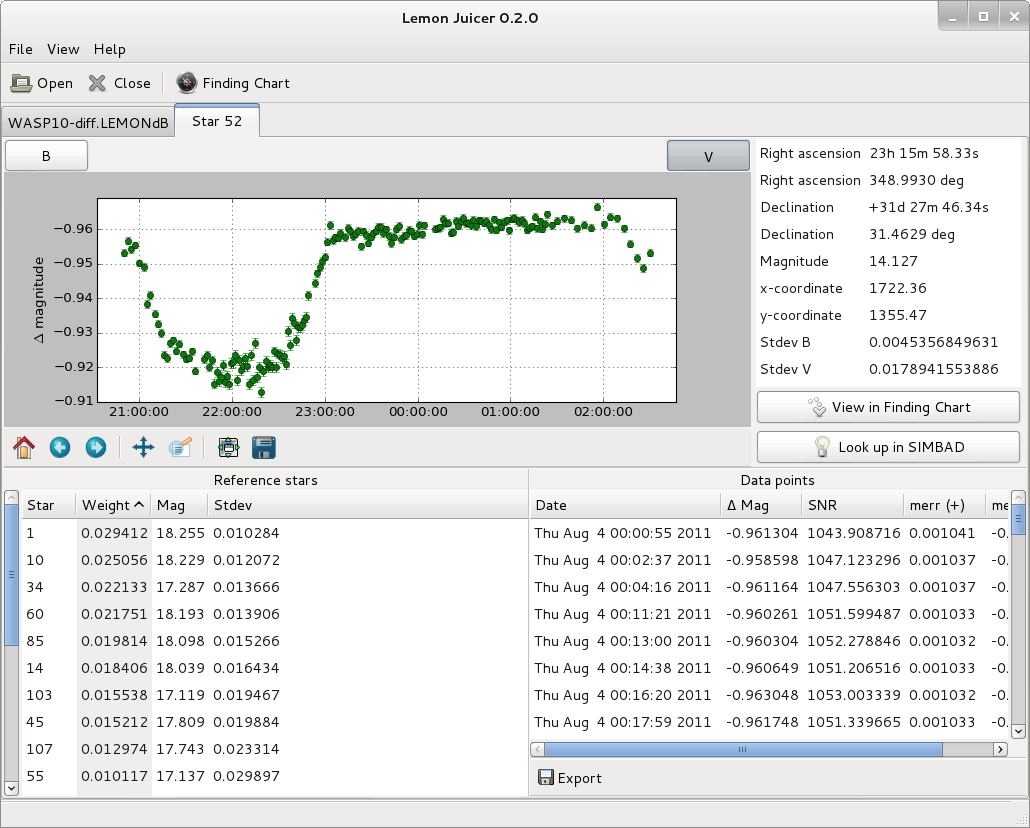
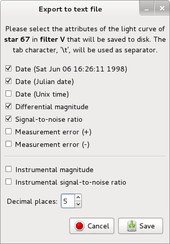
For further analysis, Export allows you save the raw data, from
which each light curve is plotted, to a text file. You can select the
fields that for each photometric measurement are written to the
file. There are three different formats available for the date:
Julian days, Unix time and a textual representation.
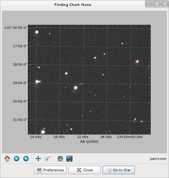
The Finding Chart button allows you to visually select the object
that you are interested in, instead of having to examine the list
trying to find it. Right-click on any point of the sky and the closest
astronomical object will be marked in red. After that, Go to Star
takes you to a window like the above, with all its data. You can, of
course, use the matplotlib interactive navigation toolbar to pan,
zoom, move back and forward, et cetera.